Advanced Robotics
- 1. Basic Concepts
- 2. Robotic Arm Motion Control
1. Basic Concepts
1.1. Terms
Configuration (构型) is a specification of the positions of all points of the robot. There are two examples that can help to explain:
- Using angles to represent the configuration of a revolving door.
- Use coordinates to represent the configuration of points on a 2D plane.
The Configuration Space (or C-space) is a n-dimensional space of all possible configurations of the robot system. The configuration of a robot is represented by a point in its C-space. Links is defined as the constructions that connect robot rigid bodies. Joints make the relative motion between adjacent links possible.
Workspace describes a set of points that can be reached by the end-effector. Two mechanisms with different C-spaces may have the same workspace, while two mechanisms with the same C-space may also have different workspaces.

Degrees of Freedom (DoF) presents the minimum number of real-valued coordinates needed to represent the configuration. For example: Spatial rigid body has 6 DoFs in 3D space; Planar rigid body has 3 DoFs in 2D plane. DoF of rigid robots = (sum of freedoms of all bodies) - (number of independent constraints). Below shows typical robot joints and their DoF:
 |
 |
|---|
Fully Actuated means all joints (DoFs) are active, Under-Actuated means at least one joint (DoF) is passive. If a manipulator has more DOF than the required task, it is called redundant (冗余的).
Serial Manipulator (串联机械手): several bodies are serially connected as a chain (open kinematic chain). For example, the normal robotic arm.
Parallel Manipulator (并联机械手): consist of several serial chains which usually support a single platform or end-effector (closed kinematic chain).

1.2. Pose of a Rigid Body
First, to describe the pose of a rigid body, we need a coordinate system. Normally, there are two coordinate systems, Left-handed system and Right-handed system. An important difference is that when describing the angle of rotation, the direction of the two is different.

The Representation of Position:
$O'$ is a point on the rigid body, which is expressed by the following relation (with respect to the coordinate frame $O-xyz$):
$$
\vec{O'} = O'_x \vec{x} + O'_y \vec{y} + O'_z \vec{z}
$$
where $O'_x, O'_y, O'_z$ denote the components of the vector $\vec{O'} \in \mathbb{R}^3$. $\vec{x}, \vec{y}, \vec{z}$ are vector.
Also, the position of $\vec{O'}$ can be compactly written as a 3 by 1 vector. $$ \vec{O'} = \left[ \begin{matrix} O'_x \\ O'_y \\ O'_z \end{matrix} \right] $$
The Representation of Orientation:
In order to describe the rigid body orientation, it is convenient to consider an orthonormal frame attached to the body, and express its unit vectors with respect to the reference frame.
Let then $O'-x'y'z'$ be such a frame with origin in $O'$, and $\vec{x'}, \vec{y'}, \vec{z'}$ be the unit vectors of the frame axes. So we have $$ \begin{aligned} \vec{x'} &= x'_x\vec{x} + x'_y\vec{y} + x'_z\vec{z} \\ \vec{y'} &= y'_x\vec{x} + y'_y\vec{y} + y'_z\vec{z} \\ \vec{z'} &= z'_x\vec{x} + z'_y\vec{y} + z'_z\vec{z} \end{aligned} $$
1.3. Rotation Matrix
By adopting a compact notation, the three unit vectors in $O'-x'y'z'$ can be combined in the 3 by 3 matrix: $$ \begin{aligned} R &= \left[ \begin{matrix} \vec{x'} & \vec{y'} & \vec{z'} \end{matrix} \right] \\ &= \left[ \begin{matrix} x'_x & y'_x & z'_x \\ x'_y & y'_u & z'_u \\ x'_z & y'_z & z'_z \end{matrix} \right] \\ &= \left[ \begin{matrix} \vec{x'}^\mathsf{T}\vec{x} & \vec{y'}^\mathsf{T}\vec{x} & \vec{z'}^\mathsf{T}\vec{x} \\ \vec{x'}^\mathsf{T}\vec{y} & \vec{y'}^\mathsf{T}\vec{y} & \vec{z'}^\mathsf{T}\vec{y} \\ \vec{x'}^\mathsf{T}\vec{z} & \vec{y'}^\mathsf{T}\vec{z} & \vec{z'}^\mathsf{T}\vec{z} \end{matrix} \right] \end{aligned} $$
where $\vec{x'}^\mathsf{T}\vec{x}$ can be considered as the projected component (投影分量) of $\vec{x'}$ on $\vec{x}$, other elements are simile.
Note: $R$ has property: $R^\mathsf{T} = R^{-1}$, so we have $p = Rp' \rightarrow p' = R^\mathsf{T}p$
Hence, when the reference frame is rotated by an angle $\alpha$ about axis $x$,$y$ and $z$, the rotation matrix of frame $O–x'y'z'$ with respect to reference frame $O–xyz$ are respectively: $$ R_x(\alpha) = \left[ \begin{matrix} 1 & 0 & 0 \\ 0 & \cos\alpha & -\sin\alpha \\ 0 & \sin\alpha & \cos\alpha \end{matrix} \right] $$ $$ R_y(\alpha) = \left[ \begin{matrix} \cos\alpha & 0 & \sin\alpha \\ 0 & 1 & 0 \\ -\sin\alpha & 0 & \cos\alpha \end{matrix} \right] $$ $$ R_z(\alpha) = \left[ \begin{matrix} \cos\alpha & -\sin\alpha & 0 \\ \sin\alpha & \cos\alpha & 0 \\ 0 & 0 & 1 \end{matrix} \right] $$
In addition, it is easy to verify that $$ \begin{aligned} R_x(-\alpha) = R_x^\mathsf{T}(\alpha) \\ R_y(-\alpha) = R_y^\mathsf{T}(\alpha) \\ R_z(-\alpha) = R_z^\mathsf{T}(\alpha) \end{aligned} $$
1.4. Rotation of a Vector
Assuming we rotate a vector under the same frame.

Solution:
First, we set the angle between $\vec{p'}$ and $x$-axis as $\beta$, the magnitude of the vector as $L$ (we know that the magnitudes of $\vec{p}$ and $\vec{p'}$ are equal). Then, we have $$ \begin{aligned} p'_x &= L*\cos\beta \\ p'_y &= L*\sin\beta \\ p_x &= L*\cos(\beta + \alpha) \\ p_y &= L*\sin(\beta + \alpha) \end{aligned} $$
According to Trigonometric Identities, we have $$ \begin{aligned} p_x &= L*\cos\beta \cos\alpha - \sin\beta \sin\alpha \\ p_y &= L*\sin\beta \cos\alpha + \cos\beta \sin\alpha \end{aligned} $$
thus, $$ \begin{aligned} p_x &= p_x'\cos\alpha - p_y' \sin\alpha \\ p_x &= p_x'\sin\alpha + p_y' \cos\alpha \\ p_z &= p'_z \end{aligned} $$
$$ \vec{p} = R_z(\alpha)\vec{p'} $$Summary:
A rotation matrix $R$ attains three equivalent geometrical meanings:
- It describes the mutual orientation between two coordinate frames; its column vectors are the direction cosines of the axes of the rotated frame with respect to the original frame.
- It represents the coordinate transformation between the coordinates of a point expressed in two different frames (with common origin).
- It is the operator that allows the rotation of a vector in the same coordinate frame.
Composition of Rotation Matrices:
- Right multiplication in rotation Matrices - rotation relative to its own (current) frame.
- Left multiplication in rotation Matrices - rotation relative to a fixed (reference) frame.
1.5. Euler Angles
Euler Angles: minimal representation of orientation $$ \phi = \left[ \begin{matrix} \varphi & \vartheta & \psi \end{matrix} \right]^\mathsf{T} $$
Euler Angles: ZYZ Angles (Intrinsic / Dynamic Euler angles):

The rotation described by ZYZ angles is obtained as composition of the following elementary rotation:
- Rotate the reference frame by the angle $\varphi$ about axis $z$
- Rotate the current frame by the angle $\vartheta$ about axis $y'$
- Rotate the current frame by the angle $\psi$ about axis $z''$
$$ R_y(\alpha) = \left[ \begin{matrix} \cos\alpha & 0 & \sin\alpha \\ 0 & 1 & 0 \\ -\sin\alpha & 0 & \cos\alpha \end{matrix} \right] $$ $$ R_z(\alpha) = \left[ \begin{matrix} \cos\alpha & -\sin\alpha & 0 \\ \sin\alpha & \cos\alpha & 0 \\ 0 & 0 & 1 \end{matrix} \right] $$When current rotation is based on previous rotation (current frame), we use symbol ($'$) to represent it.
So that, we have $$ \begin{aligned} R(\phi) &= R_{z}(\varphi)R_{y'}(\vartheta)R_{z''}(\psi) \\ &= \left[ \begin{matrix} \cos\varphi & -\sin\varphi & 0 \\ \sin\varphi & \cos\varphi & 0 \\ 0 & 0 & 1 \end{matrix} \right] \cdot \left[ \begin{matrix} \cos\vartheta & 0 & \sin\vartheta \\ 0 & 1 & 0 \\ -\sin\vartheta & 0 & \cos\vartheta \end{matrix} \right] \cdot \left[ \begin{matrix} \cos\psi & -\sin\psi & 0 \\ \sin\psi & \cos\psi & 0 \\ 0 & 0 & 1 \end{matrix} \right] \\ &= \left[ \begin{matrix} \cos\varphi \cos\vartheta & -\sin\varphi & \cos\varphi \sin\vartheta \\ \sin\varphi \cos\vartheta & \cos\varphi & \sin\varphi \sin\vartheta \\ -\sin\vartheta & 0 & \cos\vartheta \end{matrix} \right] \cdot \left[ \begin{matrix} \cos\psi & -\sin\psi & 0 \\ \sin\psi & \cos\psi & 0 \\ 0 & 0 & 1 \end{matrix} \right] \\ &= \left[ \begin{matrix} \cos\varphi \cos\vartheta \cos\psi - \sin\varphi \sin\psi & - \cos\varphi \cos\vartheta \sin\psi - \sin\varphi \cos\psi & \cos\varphi \sin\vartheta \\ \sin\varphi \cos\vartheta \cos\psi + \cos\varphi \sin\psi & - \sin\varphi \cos\vartheta \sin\psi + \cos\varphi \cos\psi & \sin\varphi \sin\vartheta \\ -\sin\vartheta \cos\psi& \sin\vartheta \sin\psi & \cos\vartheta \end{matrix} \right] \end{aligned} $$
It is useful to solve the inverse problem, that is to determine the set of Euler angles corresponding to a given rotation matrix
$$ R(\phi) = \left[ \begin{matrix} r_{11} & r_{12} & r_{13} \\ r_{21} & r_{22} & r_{23} \\ r_{31} & r_{32} & r_{33} \end{matrix} \right] $$By considering the elements $r_{13}$ and $r_{23}$, under the assumption that $r_{13} \neq 0$ and $r_{23} \neq 0$, it follows that $$ \varphi = Atan2(r_{23}, r_{13}) = Atan2 \left(\frac{\sin\varphi \sin\vartheta}{\cos\varphi \sin\vartheta}\right) $$
The function $Atan2(y, x)$ computes the arctangent of the ratio $(y/x)$ but utilizes the sign of each argument to determine which quadrant the resulting angle belongs to; this allows the correct determination of an angle in a range of $2\pi$. $$ Atan2(y,x) = \begin{cases} \arctan(y/x), &x>0 \\ \arctan(y/x)+\pi, &y\geq0,x<0 \\ \arctan(y/x)-\pi, &y<0,x<0 \\ \pi/2, &y>0,x=0 \\ -\pi/2, &y<0,x=0 \\ undefined, &y=0,x=0 \end{cases} $$
Similily, we can get $$ \begin{aligned} \vartheta &= Atan2(\sqrt{r^2_{13} + r^2_{23}}, r_{33}) \\ \psi &= Atan2(r_{32}, -r_{31}) \end{aligned} $$
where, the choice of the positive sign for the term $\sqrt{r^2_{13} + r^2_{23}}$ limits the range of feasible values of $\vartheta$ to $(0, \pi)$.
It is possible to derive another solution which produces the same effects.
Euler Angles: ZYX/RPY Angles (Extrinsic / Static Euler Angles):
Please note the rotation order.
The rotation described by RPY angles is obtained as composition of the following elementary rotation:
- Rotate the reference frame by the angle $\psi$ about axis $x$ (yaw)
- Rotate the reference frame by the angle $\vartheta$ about axis $y$ (pitch)
- Rotate the reference frame by the angle $\varphi$ about axis $z$ (roll)
So that, we have $$ \begin{aligned} R(\phi) &= R_{z}(\varphi)R_{y}(\vartheta)R_{x}(\psi) \\ &= \left[ \begin{matrix} \cos\varphi & -\sin\varphi & 0 \\ \sin\varphi & \cos\varphi & 0 \\ 0 & 0 & 1 \end{matrix} \right] \cdot \left[ \begin{matrix} \cos\vartheta & 0 & \sin\vartheta \\ 0 & 1 & 0 \\ -\sin\vartheta & 0 & \cos\vartheta \end{matrix} \right] \cdot \left[ \begin{matrix} 1 & 0 & 0 \\ 0 & \cos\psi & -\sin\psi \\ 0 & \sin\psi & \cos\psi \end{matrix} \right] \\ &= \left[ \begin{matrix} \cos\varphi \cos\vartheta & -\sin\varphi & \cos\varphi \sin\vartheta \\ \sin\varphi \cos\vartheta & \cos\varphi & \sin\varphi \sin\vartheta \\ -\sin\vartheta & 0 & \cos\vartheta \end{matrix} \right] \cdot \left[ \begin{matrix} 1 & 0 & 0 \\ 0 & \cos\psi & -\sin\psi \\ 0 & \sin\psi & \cos\psi \end{matrix} \right] \\ &= \left[ \begin{matrix} \cos\varphi \cos\vartheta & \cos\varphi \sin\vartheta \sin\psi - \sin\varphi \cos\psi & \cos\varphi \sin\vartheta \cos\psi + \sin\varphi \sin\psi \\ \sin\varphi \cos\vartheta & \sin\varphi \sin\vartheta \sin\psi + \cos\varphi \cos\psi & \sin\varphi \sin\vartheta \cos\psi - \cos\varphi \sin\psi \\ -\sin\vartheta & \cos\vartheta \sin\psi & \cos\vartheta \cos\psi \end{matrix} \right] \end{aligned} $$
The same, we can get $[\varphi, \vartheta, \psi]$ by below solution. For $\vartheta$ in the range $(−\pi/2, \pi/2)$ is $$ \begin{aligned} \varphi &= Atan2(r_{21}, r_{11}) \\ \vartheta &= Atan2(- r_{31}, \sqrt{r^2_{32} + r^2_{33}}) \\ \psi &= Atan2(r_{32}, r_{33}) \end{aligned} $$
For $\vartheta$ in the range $(\pi/2, 3\pi/2)$ is $$ \begin{aligned} \varphi &= Atan2(-r_{21}, -r_{11}) \\ \vartheta &= Atan2(- r_{31}, -\sqrt{r^2_{32} + r^2_{33}}) \\ \psi &= Atan2(-r_{32}, -r_{33}) \end{aligned} $$
1.6. Singularity (奇点) or Gimbal Lock(万向锁/环架锁定)
 |
 |
|---|
Gimbal Lock problem only happend on Intrinsic (Dynamic) Euler angles.
- Intrinsic / Dynamic Euler angles: The rotation around the current frame, using right multiplication in rotation Matrices. (e.g. ZYZ Angles)
- Extrinsic / Static Euler Angles: The rotation around the reference frame, using left multiplication in rotation Matrices. (e.g. ZYX Angles)
Gimbal lock will lead the solution cannot be uniquely determined from certain rotation.
1.7. Unit Quaternions

Quaternions can overcome the drawbacks of angle/axis representation (no singularities), which is defined as: $\mathcal{Q} = \{ \eta,\vec{\epsilon} \}$, where $$ \eta = \cos \frac{\vartheta}{2} $$ $$ \vec{\epsilon} = \sin \frac{\vartheta}{2} \vec{r} $$
$\eta$ is called the scalar part of the quaternion, while $\vec{\epsilon} = [\epsilon_x \ \epsilon_y \ \epsilon_z]^\mathsf{T}$ is called the vector part of the quaternion. They are constrained by the condition $$ \eta^2 + \epsilon_x^2 + \epsilon_y^2 + \epsilon_z^2 = 1 $$
hence, the name unit quaternion.
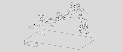
1.8. Denavit–Hartenberg convention (D-H parameters)
A good video on YouTube for learning Denavit-Hartenberg Reference Frame Layout (D-H parameters)

The D-H parameters of the above robot are
| Link | $a_i$ | $\alpha_i$ | $d_i$ | $\vartheta_i$ |
|---|---|---|---|---|
| 1 | 0 | $\pi/2$ | 0 | $\vartheta_1$ |
| 2 | $a_2$ | 0 | 0 | $\vartheta_2$ |
| 3 | 0 | $\pi/2$ | 0 | $\vartheta_3$ |
| 4 | 0 | $-\pi/2$ | $d_4$ | $\vartheta_4$ |
| 5 | 0 | $\pi/2$ | 0 | $\vartheta_5$ |
| 6 | 0 | 0 | $d_6$ | $\vartheta_6$ |
1.9. Homogeneous Transformations

In order to achieve a compact representation of the relationship between the coordinates of the same point in two different frames, the homogeneous representation of a generic vector $p$ can be introduced as the vector $\widetilde{p}$ formed by adding a fourth unit component, i.e., $$ \widetilde{p} = \left[ \begin{matrix} p \\ 1 \end{matrix} \right] $$
By adopting this representation for the vectors $p^0$ and $p^1$, the coordinate transformation can be written in terms of the (4 × 4) matrix
$$ A^0_1 = \left[ \begin{matrix} R^0_1 & o^0_1 \\ \vec{0}^\mathsf{T} & 1 \end{matrix} \right] $$This matrix is expressed in a block-partitioned form as $$ A^1_0 = \left[ \begin{matrix} {R^0_1}^\mathsf{T} & -{R^0_1}^\mathsf{T}o^0_1 \\ \vec{0}^\mathsf{T} & 1 \end{matrix} \right] = \left[ \begin{matrix} R^1_0 & -R^1_0o^0_1 \\ \vec{0}^\mathsf{T} & 1 \end{matrix} \right] $$
In general, $$ A^{-1} \neq A^\mathsf{T} $$
1.10. Direct Kinematics

With respect to a reference frame $O_b–x_by_bz_b$, the direct kinematics function is expressed by the homogeneous transformation matrix
$$ T^b_e(q) = \left[ \begin{matrix} n^b_e(q) & s^b_e(q) & a^b_e(q) & p^b_e(q) \\ 0 & 0 & 0 & 1 \end{matrix} \right] $$2. Robotic Arm Motion Control
2.1. Robot Forward Kinematics
Note: The following programs depend on the Robotics Toolbox (Matlab), please install it first.
PS: A good video on YouTube for reviewing Denavit-Hartenberg Reference Frame Layout (D-H parameters)
README:
Write a MATLAB function FK.m to compute Forward Kinematics and Geometric Jacobian for a given robot with $n$ degrees of freedom in a certain configuration. The inputs of such function should be:
- DH parameters: $n × 4$ matrix which consists of DH parameters.
- joint type: n-dimensional vector which describes joint types (0 for revolute and 1 for prismatic).
- q: n-dimensional vector of joint variables specifying the robot’s configuration.
The output of this function should be:
- T: the homogeneous transformation matrix from base to the end-effector.
- J: the Jacobian matrix of the end-effector.
2.1.1. Homogeneous Transformation Matrix
| Link | $a_i$ | $\alpha_i$ | $d_i$ | $\vartheta_i$ |
|---|---|---|---|---|
| 1 | 0 | $\pi/2$ | 0 | $\vartheta_1$ |
| 2 | $a_2$ | 0 | 0 | $\vartheta_2$ |
| 3 | 0 | $\pi/2$ | 0 | $\vartheta_3$ |
| 4 | 0 | $-\pi/2$ | $d_4$ | $\vartheta_4$ |
| 5 | 0 | $\pi/2$ | 0 | $\vartheta_5$ |
| 6 | 0 | 0 | $d_6$ | $\vartheta_6$ |
At here, the format of DH parameters is $[ a , \alpha, d, \theta]$. Meanwhile, we know the rotation matrixs $$ R_x(\alpha) = \left[ \begin{matrix} 1 & 0 & 0 \\ 0 & \cos\alpha & -\sin\alpha \\ 0 & \sin\alpha & \cos\alpha \end{matrix} \right] $$ $$ R_y(\alpha) = \left[ \begin{matrix} \cos\alpha & 0 & \sin\alpha \\ 0 & 1 & 0 \\ -\sin\alpha & 0 & \cos\alpha \end{matrix} \right] $$ $$ R_z(\alpha) = \left[ \begin{matrix} \cos\alpha & -\sin\alpha & 0 \\ \sin\alpha & \cos\alpha & 0 \\ 0 & 0 & 1 \end{matrix} \right] $$
So, we can derive the formulas $$ \begin{aligned} R_i^{i-1} &= R_z(\vartheta) * R_x(\alpha) \\ &= \left[ \begin{matrix} \cos\vartheta & -\sin\vartheta & 0 \\ \sin\vartheta & \cos\vartheta & 0 \\ 0 & 0 & 1 \end{matrix} \right] * \left[ \begin{matrix} 1 & 0 & 0 \\ 0 & \cos\alpha & -\sin\alpha \\ 0 & \sin\alpha & \cos\alpha \end{matrix} \right] \\ &= \left[ \begin{matrix} \cos\vartheta & -\sin\vartheta\cos\alpha & \sin\vartheta\sin\alpha \\ \sin\vartheta & \cos\vartheta\cos\alpha & -\cos\vartheta\sin\alpha \\ 0 & \sin\alpha & \cos\alpha \end{matrix} \right] \end{aligned} $$
Thus, we have the formula $$ A_i^{i-1} = \left[ \begin{matrix} \cos\vartheta & -\sin\vartheta\cos\alpha & \sin\vartheta\sin\alpha & a \cdot \cos\vartheta \\ \sin\vartheta & \cos\vartheta\cos\alpha & -\cos\vartheta\sin\alpha & a \cdot \sin\vartheta \\ 0 & \sin\alpha & \cos\alpha & d \\ 0 & 0 & 0 & 1 \end{matrix} \right] $$
Then we get $T_n^0$: $$ T_n^0 = A_1^0 A_2^1 ... A_n^{n-1} $$
2.1.2. Jacobian Computation
Formula:
$$ \left[ \begin{matrix} \mathcal{J}_{Pi} \\ \mathcal{J}_{Oi} \end{matrix} \right] = \begin{cases} \left[ \begin{matrix} \vec{z}_{i-1} \\ \vec{0} \end{matrix} \right] & for\ a\ prismatic\ joint \\ \left[ \begin{matrix} \vec{z}_{i-1} \times (\vec{p}_e - \vec{p}_{i-1}) \\ \vec{z}_{i-1} \end{matrix} \right] & for\ a\ revolute\ joint \end{cases} $$In particular:
- $\vec{z}_{i-1}$ is given by the third column of the rotation matrix $R^0_{i−1}$, i.e., $$ \vec{z}_{i-1} = R^0_1(q_1) ... R^{i-2}_{i-1}(q_{i-1})\vec{z}_{0} $$
where $\vec{z}_{0} =[0, 0, 1]^\mathsf{T}$ allows the selection of the third column.
- $\vec{p}_e$ is given by the first three elements of the fourth column of the transformation matrix $T^0_e$, i.e., by expressing $\widetilde{p}_e$ in the $(4 \times 1)$ homogeneous form $$ \widetilde{p}_e = A^0_1(q_1) ... A^{n-1}_n(q_n)\widetilde{p}_0 $$
where $\widetilde{p}_0 = [\vec{p}_0,1]^\mathsf{T} = [0, 0, 0, 1]^\mathsf{T}$ allows the selection of the fourth column.
- $\vec{p}_{i-1}$ is given by the first three elements of the fourth column of the transformation matrix $T^0_{i-1}$, i.e., it can be extracted from $$ \widetilde{p}_{i-1} = A^0_1(q_1) ... A^{i-2}_{i-1}(q_{i-1})\widetilde{p}_0 $$
Note: At here, $\vec{z}_{i-1} \times (\vec{p}_e - \vec{p}_{i-1})$ means cross product, using the symbol “$\times$”.
The define of cross product is $$ \vec{u} \times \vec{v} = \left( \begin{matrix} u_1 \\ u_2 \\ u_3 \end{matrix} \right) \times \left( \begin{matrix} v_1 \\ v_2 \\ v_3 \end{matrix} \right) = \left( \begin{matrix} u_2v_3 - u_3v_2 \\ u_3v_1 - u_1v_3 \\ u_1v_2 - u_2v_1 \end{matrix} \right) $$
Or, we can express it as $$ \begin{aligned} \vec{u} \times \vec{v} &= \left| \begin{matrix} \vec{i} & \vec{j} & \vec{k} \\ u_1 & u_2 & u_3 \\ v_1 & v_2 & v_3 \end{matrix} \right| \\ &= \left| \begin{matrix} u_2 & u_3 \\ v_2 & v_3 \end{matrix} \right| \vec{i} - \left| \begin{matrix} u_1 & u_3 \\ v_1 & v_3 \end{matrix} \right| \vec{j} + \left| \begin{matrix} u_1 & u_2 \\ v_1 & v_2 \end{matrix} \right| \vec{k} \\ &= (u_2v_3 - u_3v_2)\vec{i} + (u_3v_1 - u_1v_3)\vec{j} + (u_1v_2 - u_2v_1)\vec{k} \end{aligned} $$
Example:
Consider a 3DOF RPR manipulator robot. Homogenous transformation matrices for each link are $$ A_1^0 = \left[ \begin{matrix} c_1 & 0 & -s_1 & 0 \\ s_1 & 0 & c_1 & 0 \\ 0 & -1 & 0 & I_1 \\ 0 & 0 & 0 & 1 \end{matrix} \right] $$ $$ A_2^1 = \left[ \begin{matrix} 0 & 0 & 1 & 0 \\ 1 & 0 & 0 & 0 \\ 0 & 1 & 0 & d_2 \\ 0 & 0 & 0 & 1 \end{matrix} \right] $$ $$ A_3^2 = \left[ \begin{matrix} c_3 & -s_3 & 0 & I_3c_3 \\ s_3 & c_3 & 0 & I_3s_3 \\ 0 & 0 & 1 & 0 \\ 0 & 0 & 0 & 1 \end{matrix} \right] $$
where $I_1$ and $I_3$ are constant parameters, $\theta_1$, $d_2$ and $\theta_3$ are joint variables and $s_1 = \sin(\theta_1)$, $c_1 = \cos(\theta_1)$, $s_3 = \sin(\theta_3)$, $c_3 = \cos(\theta_3)$.Calculate the geometric Jacobian of the robot’s end-effector. Clearly explain every step of your calculations for each column of the Jacobian matrix.
Answers:
First, we can get $$ \begin{aligned} A_2^0 &= A_1^0 * A_2^1 \\ &= \left[ \begin{matrix} c_1 & 0 & -s_1 & 0 \\ s_1 & 0 & c_1 & 0 \\ 0 & -1 & 0 & I_1 \\ 0 & 0 & 0 & 1 \end{matrix} \right] * \left[ \begin{matrix} 0 & 0 & 1 & 0 \\ 1 & 0 & 0 & 0 \\ 0 & 1 & 0 & d_2 \\ 0 & 0 & 0 & 1 \end{matrix} \right] \\ &= \left[ \begin{matrix} 0 & -s_1 & c_1 & -d_2s_1 \\ 0 & c_1 & s_1 & d_2c_1 \\ -1 & 0 & 0 & I_1 \\ 0 & 0 & 0 & 1 \end{matrix} \right] \end{aligned} $$ $$ \begin{aligned} A_3^0 &= A_2^0 * A_3^2 \\ &= \left[ \begin{matrix} 0 & -s_1 & c_1 & -d_2s_1 \\ 0 & c_1 & s_1 & d_2c_1 \\ -1 & 0 & 0 & I_1 \\ 0 & 0 & 0 & 1 \end{matrix} \right] * \left[ \begin{matrix} c_3 & -s_3 & 0 & I_3c_3 \\ s_3 & c_3 & 0 & I_3s_3 \\ 0 & 0 & 1 & 0 \\ 0 & 0 & 0 & 1 \end{matrix} \right] \\ &= \left[ \begin{matrix} -s_1s_3 & -s_1c_3 & c_1 & -s_1I_3s_3-d_2s_1 \\ c_1s_3 & c_1c_3 & s_1 & c_1I_3s_3+d_2c_1 \\ -c_3 & s_3 & 0 & -I_3c_3+I_1 \\ 0 & 0 & 0 & 1 \end{matrix} \right] \end{aligned} $$
according to above equations, we know $$ \begin{aligned} \vec{p}_0 &= \left[ \begin{matrix} 0 \\ 0 \\ 0 \end{matrix} \right] \\ \vec{p}_1 &= \left[ \begin{matrix} 0 \\ 0 \\ I_1 \end{matrix} \right] \\ \vec{p}_2 &= \left[ \begin{matrix} -d_2s_1 \\ d_2c_1 \\ I_1 \end{matrix} \right] \\ \vec{p}_3 &= \left[ \begin{matrix} -s_1I_3s_3-d_2s_1 \\ c_1I_3s_3+d_2c_1 \\ -I_3c_3+I_1 \end{matrix} \right] \end{aligned} $$ $$ \begin{aligned} \vec{z}_0 &= \left[ \begin{matrix} 0 \\ 0 \\ 1 \end{matrix} \right] \\ \vec{z}_1 &= \left[ \begin{matrix} -s_1 \\ c_1 \\ 0 \end{matrix} \right] \\ \vec{z}_2 &= \left[ \begin{matrix} c_1 \\ s_1 \\ 0 \end{matrix} \right] \\ \end{aligned} $$
then, we get the Jacobian matrix.
PS: I found the results seem to be wrong, I will renew later or never :)
2.1.3. Forward Kinematics Codes
FK.m
Below codes show the forward kinematics algorithm.
function [T, J] = FK(DH_params, jtype, q)
% FK calculates the forward kinematics of a manipulator
% [T, J] = FK(DH_params, jtype, q) calculates the Homogeneous
% transformation matrix from base to the end-effector (T) and also the
% end-effector Jacobian with respect to the base frame of a manipulator
% robot.  The inputs are DH_params, jtype and q.  DH_params is nx4 matrix
% including Denavit-Hartenberg parameters of the robot.  jtype and q are
% n-dimensional vectors.  jtype describes the joint types of the robot.
% Its values are either 0 for revolute or 1 for prismatic joints.  q is the
% vector of joint values.


% DH = [ a, alpha, d, theta]


n = size(q,1);  % robot's DoF
% consistency check
if (n~=size(DH_params,1)) || (n~=size(jtype,1))
    error('inconsistent in dimensions');
end

% initialisation
T = eye(4,4);
J = zeros(6,n);

P = zeros(3,n+1);
Z = zeros(3,n);
Z(3,1) = 1;
%% T homogeneous matrix calculations
for i = 1:n
    if jtype(i)==0  && DH_params(i,3) ~= 0 % revolute
        error('wrong value d of the ' + i +' joint, because this is a revolute joint');
    end

    A11 = cos(q(i));
    A12 = - sin(q(i)) * cos(DH_params(i,2));
    A13 = sin(q(i)) * sin(DH_params(i,2));
    A14 = DH_params(i,1) * cos(q(i));

    A21 = sin(q(i));
    A22 = cos(q(i)) * cos(DH_params(i,2));
    A23 = -cos(q(i)) * sin(DH_params(i,2));
    A24 = DH_params(i,1) * sin(q(i));

    A31 = 0;
    A32 = sin(DH_params(i,2));
    A33 = cos(DH_params(i,2));
    A34 = DH_params(i,3);

    A = [A11,A12, A13, A14;
        A21,A22, A23, A24;
        A31,A32, A33, A34;
        0, 0, 0, 1];

    T = T * A;
    P(:,i+1) = T(1:3,4);
    Z(:,i+1) = T(1:3,3);
end

%% J Jacobian calculations
for i = 1:n
    if jtype(i)==1  %prismatic
        J(1:3,i) = Z(:,i);
        J(4:6,i) = [0,0,0];
    else             % revolute
        J(1:3,i) = crossProduct(Z(:,i), (P(:,n+1)  - P(:,i)) );
        J(4:6,i) = Z(:,i);
    end
end
end


%% calculate cross product
function c = crossProduct(u,v)
c(1) = u(2) * v(3) - u(3) * v(2);
c(2) = u(3) * v(1) - u(1) * v(3);
c(3) = u(1) * v(2) - u(2) * v(1);
end
FK_test.m
If you want to test the result of these codes, you can run below codes.
clear all;close all;clc;
%% TEST example
% This scripts is an example of how your code will be tested. sim_robot plot
% the robot in the 3D space given the DH parameters and the joint
% configuration. You can use the simulation for visual inspection purposes
% in both questions.

% DH parameters format based on Siciliano's book:
%
%      | a_1 | alpha_1 | d_1 | theta_1 |
% DH = | ... | ....... | ... | ....... |
%      | a_n | alpha_n | d_n | theta_n |
%
% with alpha_i and theta_i in radiant
%% EXAMPLE: planar robot
q = [pi/2;pi/4;pi/2];

DH(:,1) = [0.5 1 0.5]';             % a
DH(:,2) = [0 0 0]';           % alpha
DH(:,3) = [0 0 0]';               % d
DH(:,4) = q;      % theta

jtype = zeros(3,1);

% Forward Kinematics
[T1, J1] = FK(DH, jtype, q);

% Plot robot
figure()
sim_robot(DH,q,jtype)

%% Other examples
% set up here the code to test your FK function with other robot's
% configuration/DH parameters
2.2. Robot Inverse Kinematics
Note: The following programs depend on the Robotics Toolbox (Matlab), please install it first.
PS: A good video on YouTube for reviewing Denavit-Hartenberg Reference Frame Layout (D-H parameters)
There is a RRR manipulator schematic diagram showed below. Following examples will be based on this illustration.
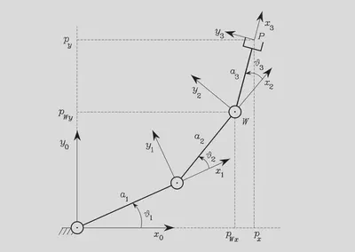
Assuming that we know $(p_{Wx} , p_{Wy})$, $a_1$ and $a_2$. We need to solve $\vartheta_1$ and $\vartheta_2$.
2.2.1. Geometry Solution
Based on geometry knowledge, we can get $$ p_{Wx}^2 + p_{Wy}^2 = a_1^2 + a_2^2 - 2a_1a_2\cos(180^{\circ} - \vartheta_2) $$
Then, we have $$ \cos \vartheta_2 = \frac{p_{Wx}^2 + p_{Wy}^2 - a_1^2 - a_2^2}{2a_1a_2} $$
According to The Law of Cosines $\cos A=(b²+c²-a²)/2bc$ , we set the angle between $x_1$ and $\vec{p}_W = [p_{Wx} , p_{Wy} , 0]$ is $\psi$, then have $$ \cos \psi = \frac{p_{Wx}^2 + p_{Wy}^2 + a_1^2 - a_2^2}{2a_1\sqrt{p_{Wx}^2 + p_{Wy}^2}} $$
We get $$ \vartheta_1 = \begin{cases} atan2(p_{Wy},p_{Wx}) + \psi & \vartheta_2 < 0^{\circ} \\ atan2(p_{Wy},p_{Wx}) - \psi & \vartheta_2 > 0^{\circ} \end{cases} (0^{\circ} < \psi < 180^{\circ}) $$
2.2.2. Algebraic Solution
Now, we show the homogeneous transformation matrixs, $$ \begin{aligned} T_2^0 &= T_1^0T_2^1 \\ &= \left[ \begin{matrix} \cos \vartheta_1 & -\sin \vartheta_1 & 0 & a_1\cos \vartheta_1 \\ \sin \vartheta_1 & \cos \vartheta_1 & 0 & a_1\sin \vartheta_1 \\ 0 & 0 & 1 & 0 \\ 0 & 0 & 0 & 1 \end{matrix} \right] \left[ \begin{matrix} \cos \vartheta_2 & -\sin \vartheta_2 & 0 & a_2\cos \vartheta_2 \\ \sin \vartheta_2 & \cos \vartheta_2 & 0 & a_2\sin \vartheta_2 \\ 0 & 0 & 1 & 0 \\ 0 & 0 & 0 & 1 \end{matrix} \right] \\ &= \left[ \begin{matrix} \cos (\vartheta_1 + \vartheta_2) & -\sin (\vartheta_1 + \vartheta_2) & 0 & a_2\cos (\vartheta_1 + \vartheta_2) + a_1 \cos \vartheta_1 \\ \sin (\vartheta_1 + \vartheta_2) & \cos (\vartheta_1 + \vartheta_2) & 0 & a_2\sin (\vartheta_1 + \vartheta_2) + a_1 \sin \vartheta_1 \\ 0 & 0 & 1 & 0 \\ 0 & 0 & 0 & 1 \end{matrix} \right] \\ &= \left[ \begin{matrix} \cos \phi & -\sin \phi & 0 & p_{Wx} \\ \sin \phi & \cos \phi & 0 & p_{Wy} \\ 0 & 0 & 1 & 0 \\ 0 & 0 & 0 & 1 \end{matrix} \right] \end{aligned} $$
We can know $$ \begin{aligned} p_{Wx}^2 + p_{Wy}^2 &= (a_2\cos (\vartheta_1 + \vartheta_2) + a_1 \cos \vartheta_1)^2 + (a_2\sin (\vartheta_1 + \vartheta_2) + a_1 \sin \vartheta_1)^2 \\ &= a_2^2 \cos^2 (\vartheta_1 + \vartheta_2) + a_1^2 \cos^2 \vartheta_1 + 2 a_1 a_2 \cos (\vartheta_1 + \vartheta_2) \cos \vartheta_1 + a_2^2 \sin^2 (\vartheta_1 + \vartheta_2) + a_1^2 \sin^2 \vartheta_1 + 2 a_1 a_2 \sin (\vartheta_1 + \vartheta_2) \sin \vartheta_1 \\ &= a_1^2 + a_2^2 + 2 a_1 a_2 \cos \vartheta_2 \end{aligned} $$
We get $$ \cos \vartheta_2 = \frac{p_{Wx}^2 + p_{Wy}^2 - a_1^2 - a_2^2}{2a_1a_2} $$
-
If $\cos \vartheta_2 > 1$ or $\cos \vartheta_2 < -1$: too far for the manipulator to reach.
-
If $-1 \leq \cos \vartheta_2 \leq 1$: two solutions.
Now, we have known $\vartheta_2$, $a_1$ and $a_2$. So we have $$ \begin{aligned} p_{Wx} &= a_2\cos (\vartheta_1 + \vartheta_2) + a_1 \cos \vartheta_1 \\ &= (a_1 + a_2 \cos \vartheta_2)\cos \vartheta_1 + (-a_2 \sin \vartheta_2)\sin \vartheta_1 \\ p_{Wy} &= a_2\sin (\vartheta_1 + \vartheta_2) + a_1 \sin \vartheta_1 \\ &= (a_1 + a_2 \cos \vartheta_2)\sin \vartheta_1 + (a_2 \sin \vartheta_2)\cos \vartheta_1 \end{aligned} $$
Because $\vartheta_2$, $a_1$ and $a_2$ are known, so we set $$ k_1 = a_1 + a_2 \cos \vartheta_2 \\ k_2 = a_2 \sin \vartheta_2 $$
Above functions became (Note: $k_1$ and $k_2$ are constant) $$ p_{Wx} = k_1 \cos \vartheta_1 - k_2 \sin \vartheta_1 \\ p_{Wy} = k_1 \sin \vartheta_1 + k_2 \cos \vartheta_1 $$
Next, we define $$ r = \sqrt{k_1^2 + k_2^2} \\ \gamma = atan2(k_2,k_1) $$
and we have $$ k_1 = r \cos\gamma \\ k_2 = r \sin\gamma $$
then we can get $$ \begin{aligned} \frac{p_{Wx}}{r} &= \frac{k_1 \cos \vartheta_1 - k_2 \sin \vartheta_1}{r} \\ &= \frac{r \cos\gamma \cos\vartheta_1 - r \sin\gamma \sin\vartheta_1}{r} \\ &= \cos\gamma \cos\vartheta_1 - \sin\gamma \sin\vartheta_1 \\ &= \cos(\gamma + \vartheta_1) \end{aligned} $$
in the same way $$ \frac{p_{Wy}}{r} = \sin(\gamma + \vartheta_1) $$
finally, we get $$ \gamma + \vartheta_1 = atan2(\frac{p_{Wy}}{r} , \frac{p_{Wx}}{r}) = atan2(p_{Wy} , p_{Wx}) $$
i.e. $$ \vartheta_1 = atan2(p_{Wy} , p_{Wx}) - atan2(k_2 , k_1) $$
2.2.3. Solve Trigonometric Equations
For example, we assume that there is an equation, $a \cos\theta + b \sin\theta = c$, we need to solve $\theta$.
First, we set $$ \tan(\frac{\theta}{2}) = \mu ,\ \cos(\theta) = \frac{1 - \mu^2}{1 + \mu^2} ,\ \sin(\theta) = \frac{2\mu}{1 + \mu^2} $$
now we have $$ \begin{align} &a \frac{1 - \mu^2}{1 + \mu^2} + b \frac{2\mu}{1 + \mu^2} = c \\ &(a+c)\mu^2 -2b\mu + (c-a) = 0 \end{align} $$
$$ \mu = \frac{b \pm \sqrt{b^2 + a^2 - c^2}}{a+c} $$2.3. Generic Inverse Kinematics Algorithm
README:
Write a MATLAB function IK.m to solve for the iterative Inverse Kinematics of a given robot. The inputs of this function should be:
- DH parameters: $n × 4$ matrix which consists of DH parameters.
- joint type: n-dimensional vector which describes joint types (0 for revolute and 1 for prismatic).
- q: n-dimensional vector of joint variables specifying the robot’s configuration.
- desired position: desired position of the robot’s end-effector. This is $2 \times 1$ vector for a planar robot and $3 \times 1$ vector for a spatial robot.
- desired orientation: desired orientation of the robot’s end-effector. This is a scalar for a planar robot and a $3 \times 1$ vector for a spatial robot. Use roll-pitch-yaw angles for 3D robots.
IK can be implemented using the Jacobian Transpose to compute the inverse of the Jacobian matrix. The output of the IK function should be:
- a matrix including the robot’s joint variables for each iteration.
Note that, this function solve the IK problem iteratively. So, you need to define appropriate terminating conditions for both maximum iterations and accuracy of the final result. When updating joint variables, consider multiplying by a small gain in order to let the algorithm converge. Use the script IK_test.m to define your robot, solve the IK problem, and visualize how the robot achieves the desired end-effector pose.
2.3.1. Geometric Jacobian
As we know, for Geometric Jacobian $$ v_e = \left[ \begin{matrix} \dot{p}_e \\ \dot{w}_e \end{matrix} \right] = J(q)\dot{q} $$
where $J = \left[\begin{matrix} J_P \\ J_O \end{matrix} \right]$.
$$ \dot{q} = J^{-1}v_e $$that is $$ [\Delta \vartheta_1, \Delta \vartheta_2 ... \Delta \vartheta_n] = J^{-1} [\Delta p_x, \Delta p_y, \Delta p_z, \Delta w_x, \Delta w_y, \Delta w_z] $$
i.e. $$ [\frac{\vartheta_1}{t}, \frac{\vartheta_2}{t} ... \frac{\vartheta_n}{t}] = J^{-1} [\frac{p_x}{t}, \frac{p_y}{t}, \frac{p_z}{t}, \frac{w_x}{t}, \frac{w_y}{t}, \frac{w_z}{t}] $$
where $\vartheta$ corresponds to the angle of joints, $p$ and $w$ corresponds to the position and orientation of the end-effector.
2.3.2. Analytical Jacobian
For Analytical Jacobian $$ \dot{x}_e = \left[ \begin{matrix} \dot{p}_e \\ \dot{\phi}_e \end{matrix} \right] = \left[\begin{matrix} J_P(q) \\ J_\phi(q) \end{matrix} \right] \dot{q} = J_A(q)\dot{q} $$
$$ \dot{q} = J_A^{-1}\dot{x}_e $$that is $$ [\Delta \vartheta_1, \Delta \vartheta_2 ... \Delta \vartheta_n] = J^{-1} [\Delta p_x, \Delta p_y, \Delta p_z, \Delta \psi, \Delta \vartheta, \Delta \varphi] $$
i.e. $$ [\frac{\vartheta_1}{t}, \frac{\vartheta_2}{t} ... \frac{\vartheta_n}{t}] = J^{-1} [\frac{p_x}{t}, \frac{p_y}{t}, \frac{p_z}{t}, \frac{\psi}{t}, \frac{\vartheta}{t}, \frac{\varphi}{t}] $$
where $\vartheta$ corresponds to the angle of joints, $p$ corresponds to the position of the end-effector, $[\psi , \vartheta , \varphi]$ corresponds to the [yaw, pitch, yaw](RPY Angles system) respectively.
2.3.3. Jacobian Pseudo-inverse (generalized inverse)
Set the size of Jacobian is $[n,m]$, them we have:
-
when $n>m$, we use left generalized inverse $$ A^\dagger_{left} = (A^\mathsf{T}A)^{-1}A^\mathsf{T} $$
-
when $n
2.3.4. Kinematic Singularities
For Kinematic Singularities, we set a small value of $k$ to let the algorithm converge. (Damped least squares) $$ J^* = J^\mathsf{T}(J J^\mathsf{T} + k^2I)^{-1} $$
normally, we set $k = 0.01$.
2.3.5. Inverse Kinematics Codes
Algorithm Overview:
we set:
$\theta_k:$ initial joint angles
$p_{des}:$ desired position
$o_{des}:$ desired orientation
$t:$ Hypothetical robot movement time
- We get the homogeneous transformation matrix $T_k$ form $\theta_k$.
- Calculate the position $p_k$ and oritention $w_k$ of the end-effector.
- We approximate the velocity of end effector movement $v_k = ([p_{des}, o_{des}] - [p_k, w_k]) ./ t$
- Get Joint Angle Increment $\Delta \theta = J_k^{-1} * v_k$
- Update joint angles $\theta_{k+1} = \theta_k + \Delta \theta$
- Calculation error, determining whether to continue iterating.
IK.m
Below codes show the inverse kinematics algorithm.
function Q = IK(DH_params, jtype, q, pdes, odes)
% IK calculates the inverse kinematics of a manipulator
% Q = IK(DH_params, jtype, q, pdes, odes) calculates the joint
% values of a manipulator robot given the desired end-effector's position
% and orientation by solving the inverse kinematics, iteratively.  The
% inputs are DH_params, jtype and q, pdes, and odes.  DH_params is
% nx4 matrix including Denavit-Hartenberg parameters of the robot.  jtype
% and q are n-dimensional vectors.  jtype describes the joint types of the
% robot and its values are either 0 for revolute or 1 for prismatic joints.
% q is the joint values.  pdes and odes are desired position and
% orientation of the end-effector.  pdes is 2x1 for a planar robot and 3x1
% for a spatial one.  odes is a scalar for a planar robot and a 3x1 vector
% for a 3D robot.  Orientation is defined as roll-pitch-yaw angles.  Use
% Jacobian Transpose to compute the inverse of the Jacobian.

n = size(q,1);  % robot's DoF
% consistency check
if (n~=size(DH_params,1)) || (n~=size(jtype,1))
    error('inconsistent in dimensions');
end

% robot's dimension (planar or spatial)
dim = size(pdes,1);
if ~((dim==2) || (dim==3))
    error('size of pdes must be either 2x1 for a planar robot or 3x1 for a spatial robot');
end

% check the size of orientation parameter
if dim==2
    if size(odes,1)~=1
        error('desired orientation must be scalar for a planar robot');
    end
else
    if size(odes,1)~=3
        error('desired orientation must be 3x1 for a spatial robot');
    end
end

%% iterative inverse kinematics


Q = q;  % joint angle
thetaK = q;  % initial joint angle
time = 100;
iTime = 0;
single = 1; % if value is 1, continue to iterate

% Calculate the oritention of the end effector in the current stage
[TCur_k,J_k] = FK(DH_params, jtype, q);
o_e = oEnd(TCur_k(1:3,1:3));

% Approximate end-effector velocity, determine the direction of movement
dX = ([pdes; odes] - [TCur_k(1:3,4); o_e]) ./ time;


JTranspose = IKJ(J_k);
dO = JTranspose *  dX; % Variation of joint angles

while single

    iTime = iTime +1;
    thetaK1 = dO + thetaK;

    % Calculate the oritention of the end effector in the next stage
    [TCur_k1,J_k1] = FK(DH_params, jtype, thetaK1);
    o_e1 = oEnd(TCur_k1(1:3,1:3));

    % calculate the error
    e = sum(sum(abs([TCur_k1(1:3,4); o_e1] - [pdes; odes])));
    if e<0.1 || iTime>= time
        single = 0; % stoping iterating
    end

    thetaK = thetaK1;
    JTranspose = IKJ(J_k1);
    dO = JTranspose *  dX; % Variation of joint angles

    Q = [Q,thetaK];
end

end


%% IKJ
% Pseudo-Inverse Matrix Solving
function JTranspose = IKJ(J)

[n,m] = size(J);
k = 0.01; % Avoid singular solutions

if n>m
    JTranspose = (J' * J + k^2 .* eye(m,m)) \ J';
else
    JTranspose = J' / (J  * J' + k^2 .* eye(n,n));
end

end


%% oEnd
% Convert rotation matrix to angles of end effector
function o = oEnd(R)

o = zeros(3,1);

% x
o(3) = atan2(R(2,1), R(1,1));
% y
o(2) = atan2(-R(3,1), sqrt(R(3,2)^2 + R(3,3)^2));
% z
o(1) = atan2(R(3,2), R(3,3));
end
IK_test.m
If you want to test the result of these codes, you can run below codes.
clear all;close all;clc;
%% TEST example
% This scripts is an example of how your code will be tested. sim_robot plot
% the robot in the 3D space given the DH parameters and the joint
% configuration. You can use the simulation for visual inspection purposes
% in both questions.

% DH parameters format based on Siciliano's book:
%
%      | a_1 | alpha_1 | d_1 | theta_1 |
% DH = | ... | ....... | ... | ....... |
%      | a_n | alpha_n | d_n | theta_n |
%
% with alpha_i and theta_i in radiant
%% EXAMPLE 1: Three-link Planar Arm
q = rand(3,1) * (pi/2);
jtype = [0;0;0];
DH(:,1) = rand(3,1);            % a
DH(:,2) = zeros(3,1);           % alpha
DH(:,3) = zeros(3,1);           % d
DH(:,4) = q;                    % theta

q_des = rand(3,1) * (pi/2);              % desired joint configuration
[T,~] = FK(DH, jtype, q_des);
p_des = T(1:3,4);               % desired end-effector configuration
R = T(1:3,1:3);
phi_des = oEnd(R);

Q = IK(DH, jtype, q, p_des, phi_des);

figure()
plot(transpose(Q))
xlabel('num iter')
ylabel('q')
legend('q_1','q_2','q_3');

[T,~] = FK(DH, jtype, Q(:,end));

pfinal = T(1:3,4);
R = T(1:3,1:3);
phifinal = oEnd(R);

% Check the final error between the current end-effector pose and the desired one
p_error = p_des-pfinal
o_error = phi_des-phifinal

% Simulate the robot at each step of the iterative inverse kinematics and observe how the end-effector reaches the desired pose
figure()
for steps = 1:size(Q,2)
    sim_robot(DH,Q(:,steps),jtype)
end


%% oEnd
function o = oEnd(R)
o = zeros(3,1);

o(3) = atan2(R(2,1), R(1,1));
o(2) = atan2(-R(3,1), sqrt(R(3,2)^2 + R(3,3)^2));
o(1) = atan2(R(3,2), R(3,3));
end