1. Robot Forward Kinematics

Note: The following programs depend on the Robotics Toolbox (Matlab), please install it first.

PS: A good video on YouTube for reviewing Denavit-Hartenberg Reference Frame Layout (D-H parameters)

1.1. Introduction

Write a MATLAB function FK.m to compute Forward Kinematics and Geometric Jacobian for a given robot with $n$ degrees of freedom in a certain configuration. The inputs of such function should be:

DH parameters: $n × 4$ matrix which consists of DH parameters.
joint type: n-dimensional vector which describes joint types (0 for revolute and 1 for prismatic).
q: n-dimensional vector of joint variables specifying the robot’s configuration.

The output of this function should be:

T: the homogeneous transformation matrix from base to the end-effector.
J: the Jacobian matrix of the end-effector.

1.2. Theoretical Derivation

1.2.1. Homogeneous Transformation Matrix

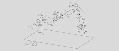
Link	$a_i$	$\alpha_i$	$d_i$	$\vartheta_i$
1	0	$\pi/2$	0	$\vartheta_1$
2	$a_2$	0	0	$\vartheta_2$
3	0	$\pi/2$	0	$\vartheta_3$
4	0	$-\pi/2$	$d_4$	$\vartheta_4$
5	0	$\pi/2$	0	$\vartheta_5$
6	0	0	$d_6$	$\vartheta_6$

At here, the format of DH parameters is $[ a , \alpha, d, \theta]$. Meanwhile, we know the rotation matrixs $$ R_x(\alpha) = \left[ \begin{matrix} 1 & 0 & 0 \\ 0 & \cos\alpha & -\sin\alpha \\ 0 & \sin\alpha & \cos\alpha \end{matrix} \right] $$ $$ R_y(\alpha) = \left[ \begin{matrix} \cos\alpha & 0 & \sin\alpha \\ 0 & 1 & 0 \\ -\sin\alpha & 0 & \cos\alpha \end{matrix} \right] $$ $$ R_z(\alpha) = \left[ \begin{matrix} \cos\alpha & -\sin\alpha & 0 \\ \sin\alpha & \cos\alpha & 0 \\ 0 & 0 & 1 \end{matrix} \right] $$

So, we can derive the formulas $$ \begin{aligned} R_i^{i-1} &= R_z(\vartheta) * R_x(\alpha) \\ &= \left[ \begin{matrix} \cos\vartheta & -\sin\vartheta & 0 \\ \sin\vartheta & \cos\vartheta & 0 \\ 0 & 0 & 1 \end{matrix} \right] * \left[ \begin{matrix} 1 & 0 & 0 \\ 0 & \cos\alpha & -\sin\alpha \\ 0 & \sin\alpha & \cos\alpha \end{matrix} \right] \\ &= \left[ \begin{matrix} \cos\vartheta & -\sin\vartheta\cos\alpha & \sin\vartheta\sin\alpha \\ \sin\vartheta & \cos\vartheta\cos\alpha & -\cos\vartheta\sin\alpha \\ 0 & \sin\alpha & \cos\alpha \end{matrix} \right] \end{aligned} $$

Thus, we have the formula $$ A_i^{i-1} = \left[ \begin{matrix} \cos\vartheta & -\sin\vartheta\cos\alpha & \sin\vartheta\sin\alpha & a \cdot \cos\vartheta \\ \sin\vartheta & \cos\vartheta\cos\alpha & -\cos\vartheta\sin\alpha & a \cdot \sin\vartheta \\ 0 & \sin\alpha & \cos\alpha & d \\ 0 & 0 & 0 & 1 \end{matrix} \right] $$

Then we get $T_n^0$: $$ T_n^0 = A_1^0 A_2^1 ... A_n^{n-1} $$

1.2.2. Jacobian Computation

1.2.2.1. Formula

$$ \left[ \begin{matrix} \mathcal{J}_{Pi} \\ \mathcal{J}_{Oi} \end{matrix} \right] = \begin{cases} \left[ \begin{matrix} \vec{z}_{i-1} \\ \vec{0} \end{matrix} \right] & for\ a\ prismatic\ joint \\ \left[ \begin{matrix} \vec{z}_{i-1} \times (\vec{p}_e - \vec{p}_{i-1}) \\ \vec{z}_{i-1} \end{matrix} \right] & for\ a\ revolute\ joint \end{cases} $$

In particular:

$\vec{z}_{i-1}$ is given by the third column of the rotation matrix $R^0_{i−1}$, i.e., $$ \vec{z}_{i-1} = R^0_1(q_1) ... R^{i-2}_{i-1}(q_{i-1})\vec{z}_{0} $$

where $\vec{z}_{0} =[0, 0, 1]^\mathsf{T}$ allows the selection of the third column.

$\vec{p}_e$ is given by the first three elements of the fourth column of the transformation matrix $T^0_e$, i.e., by expressing $\widetilde{p}_e$ in the $(4 \times 1)$ homogeneous form $$ \widetilde{p}_e = A^0_1(q_1) ... A^{n-1}_n(q_n)\widetilde{p}_0 $$

where $\widetilde{p}_0 = [\vec{p}_0,1]^\mathsf{T} = [0, 0, 0, 1]^\mathsf{T}$ allows the selection of the fourth column.

$\vec{p}_{i-1}$ is given by the first three elements of the fourth column of the transformation matrix $T^0_{i-1}$, i.e., it can be extracted from $$ \widetilde{p}_{i-1} = A^0_1(q_1) ... A^{i-2}_{i-1}(q_{i-1})\widetilde{p}_0 $$

Note

At here, $\vec{z}_{i-1} \times (\vec{p}_e - \vec{p}_{i-1})$ means cross product, using the symbol “$\times$”.

The define of cross product is $$ \vec{u} \times \vec{v} = \left( \begin{matrix} u_1 \\ u_2 \\ u_3 \end{matrix} \right) \times \left( \begin{matrix} v_1 \\ v_2 \\ v_3 \end{matrix} \right) = \left( \begin{matrix} u_2v_3 - u_3v_2 \\ u_3v_1 - u_1v_3 \\ u_1v_2 - u_2v_1 \end{matrix} \right) $$

Or, we can express it as $$ \begin{aligned} \vec{u} \times \vec{v} &= \left| \begin{matrix} \vec{i} & \vec{j} & \vec{k} \\ u_1 & u_2 & u_3 \\ v_1 & v_2 & v_3 \end{matrix} \right| \\ &= \left| \begin{matrix} u_2 & u_3 \\ v_2 & v_3 \end{matrix} \right| \vec{i} - \left| \begin{matrix} u_1 & u_3 \\ v_1 & v_3 \end{matrix} \right| \vec{j} + \left| \begin{matrix} u_1 & u_2 \\ v_1 & v_2 \end{matrix} \right| \vec{k} \\ &= (u_2v_3 - u_3v_2)\vec{i} + (u_3v_1 - u_1v_3)\vec{j} + (u_1v_2 - u_2v_1)\vec{k} \end{aligned} $$

1.2.2.2. Example

Consider a 3DOF RPR manipulator robot. Homogenous transformation matrices for each link are $$ A_1^0 = \left[ \begin{matrix} c_1 & 0 & -s_1 & 0 \\ s_1 & 0 & c_1 & 0 \\ 0 & -1 & 0 & I_1 \\ 0 & 0 & 0 & 1 \end{matrix} \right] $$ $$ A_2^1 = \left[ \begin{matrix} 0 & 0 & 1 & 0 \\ 1 & 0 & 0 & 0 \\ 0 & 1 & 0 & d_2 \\ 0 & 0 & 0 & 1 \end{matrix} \right] $$ $$ A_3^2 = \left[ \begin{matrix} c_3 & -s_3 & 0 & I_3c_3 \\ s_3 & c_3 & 0 & I_3s_3 \\ 0 & 0 & 1 & 0 \\ 0 & 0 & 0 & 1 \end{matrix} \right] $$

where $I_1$ and $I_3$ are constant parameters, $\theta_1$, $d_2$ and $\theta_3$ are joint variables and $s_1 = \sin(\theta_1)$, $c_1 = \cos(\theta_1)$, $s_3 = \sin(\theta_3)$, $c_3 = \cos(\theta_3)$.Calculate the geometric Jacobian of the robot’s end-effector. Clearly explain every step of your calculations for each column of the Jacobian matrix.

Answers:

First, we can get $$ \begin{aligned} A_2^0 &= A_1^0 * A_2^1 \\ &= \left[ \begin{matrix} c_1 & 0 & -s_1 & 0 \\ s_1 & 0 & c_1 & 0 \\ 0 & -1 & 0 & I_1 \\ 0 & 0 & 0 & 1 \end{matrix} \right] * \left[ \begin{matrix} 0 & 0 & 1 & 0 \\ 1 & 0 & 0 & 0 \\ 0 & 1 & 0 & d_2 \\ 0 & 0 & 0 & 1 \end{matrix} \right] \\ &= \left[ \begin{matrix} 0 & -s_1 & c_1 & -d_2s_1 \\ 0 & c_1 & s_1 & d_2c_1 \\ -1 & 0 & 0 & I_1 \\ 0 & 0 & 0 & 1 \end{matrix} \right] \end{aligned} $$ $$ \begin{aligned} A_3^0 &= A_2^0 * A_3^2 \\ &= \left[ \begin{matrix} 0 & -s_1 & c_1 & -d_2s_1 \\ 0 & c_1 & s_1 & d_2c_1 \\ -1 & 0 & 0 & I_1 \\ 0 & 0 & 0 & 1 \end{matrix} \right] * \left[ \begin{matrix} c_3 & -s_3 & 0 & I_3c_3 \\ s_3 & c_3 & 0 & I_3s_3 \\ 0 & 0 & 1 & 0 \\ 0 & 0 & 0 & 1 \end{matrix} \right] \\ &= \left[ \begin{matrix} -s_1s_3 & -s_1c_3 & c_1 & -s_1I_3s_3-d_2s_1 \\ c_1s_3 & c_1c_3 & s_1 & c_1I_3s_3+d_2c_1 \\ -c_3 & s_3 & 0 & -I_3c_3+I_1 \\ 0 & 0 & 0 & 1 \end{matrix} \right] \end{aligned} $$

according to above equations, we know $$ \begin{aligned} \vec{p}_0 &= \left[ \begin{matrix} 0 \\ 0 \\ 0 \end{matrix} \right] \\ \vec{p}_1 &= \left[ \begin{matrix} 0 \\ 0 \\ I_1 \end{matrix} \right] \\ \vec{p}_2 &= \left[ \begin{matrix} -d_2s_1 \\ d_2c_1 \\ I_1 \end{matrix} \right] \\ \vec{p}_3 &= \left[ \begin{matrix} -s_1I_3s_3-d_2s_1 \\ c_1I_3s_3+d_2c_1 \\ -I_3c_3+I_1 \end{matrix} \right] \end{aligned} $$ $$ \begin{aligned} \vec{z}_0 &= \left[ \begin{matrix} 0 \\ 0 \\ 1 \end{matrix} \right] \\ \vec{z}_1 &= \left[ \begin{matrix} -s_1 \\ c_1 \\ 0 \end{matrix} \right] \\ \vec{z}_2 &= \left[ \begin{matrix} c_1 \\ s_1 \\ 0 \end{matrix} \right] \\ \end{aligned} $$

then, we get the Jacobian matrix.

1.2.3. Demo Codes

FK.m

Below codes show the forward kinematics algorithm.

function [T, J] = FK(DH_params, jtype, q)
% FK calculates the forward kinematics of a manipulator
% [T, J] = FK(DH_params, jtype, q) calculates the Homogeneous
% transformation matrix from base to the end-effector (T) and also the
% end-effector Jacobian with respect to the base frame of a manipulator
% robot.  The inputs are DH_params, jtype and q.  DH_params is nx4 matrix
% including Denavit-Hartenberg parameters of the robot.  jtype and q are
% n-dimensional vectors.  jtype describes the joint types of the robot.
% Its values are either 0 for revolute or 1 for prismatic joints.  q is the
% vector of joint values.


% DH = [ a, alpha, d, theta]


n = size(q,1);  % robot's DoF
% consistency check
if (n~=size(DH_params,1)) || (n~=size(jtype,1))
    error('inconsistent in dimensions');
end

% initialisation
T = eye(4,4);
J = zeros(6,n);

P = zeros(3,n+1);
Z = zeros(3,n);
Z(3,1) = 1;
%% T homogeneous matrix calculations
for i = 1:n
    if jtype(i)==0  && DH_params(i,3) ~= 0 % revolute
        error('wrong value d of the ' + i +' joint, because this is a revolute joint');
    end

    A11 = cos(q(i));
    A12 = - sin(q(i)) * cos(DH_params(i,2));
    A13 = sin(q(i)) * sin(DH_params(i,2));
    A14 = DH_params(i,1) * cos(q(i));

    A21 = sin(q(i));
    A22 = cos(q(i)) * cos(DH_params(i,2));
    A23 = -cos(q(i)) * sin(DH_params(i,2));
    A24 = DH_params(i,1) * sin(q(i));
 
    A31 = 0;
    A32 = sin(DH_params(i,2));
    A33 = cos(DH_params(i,2));
    A34 = DH_params(i,3);

    A = [A11,A12, A13, A14;
        A21,A22, A23, A24;
        A31,A32, A33, A34;
        0, 0, 0, 1];

    T = T * A;
    P(:,i+1) = T(1:3,4);
    Z(:,i+1) = T(1:3,3);
end

%% J Jacobian calculations
for i = 1:n
    if jtype(i)==1  %prismatic
        J(1:3,i) = Z(:,i);
        J(4:6,i) = [0,0,0];
    else             % revolute
        J(1:3,i) = crossProduct(Z(:,i), (P(:,n+1)  - P(:,i)) );
        J(4:6,i) = Z(:,i);
    end
end
end



%% calculate cross product
function c = crossProduct(u,v)
c(1) = u(2) * v(3) - u(3) * v(2);
c(2) = u(3) * v(1) - u(1) * v(3);
c(3) = u(1) * v(2) - u(2) * v(1);
end

FK_test.m

If you want to test the result of these codes, you can run below codes.

clear all;close all;clc;
%% TEST example
% This scripts is an example of how your code will be tested. sim_robot plot
% the robot in the 3D space given the DH parameters and the joint
% configuration. You can use the simulation for visual inspection purposes
% in both questions.

% DH parameters format based on Siciliano's book:
%
%      | a_1 | alpha_1 | d_1 | theta_1 |
% DH = | ... | ....... | ... | ....... |
%      | a_n | alpha_n | d_n | theta_n |
%
% with alpha_i and theta_i in radiant
%% EXAMPLE: planar robot
q = [pi/2;pi/4;pi/2];

DH(:,1) = [0.5 1 0.5]';             % a
DH(:,2) = [0 0 0]';           % alpha
DH(:,3) = [0 0 0]';               % d
DH(:,4) = q;      % theta

jtype = zeros(3,1);

% Forward Kinematics
[T1, J1] = FK(DH, jtype, q);

% Plot robot
figure()
sim_robot(DH,q,jtype)

%% Other examples
% set up here the code to test your FK function with other robot's
% configuration/DH parameters

2. Robot Inverse Kinematics

Note: The following programs depend on the Robotics Toolbox (Matlab), please install it first.

PS: A good video on YouTube for reviewing Denavit-Hartenberg Reference Frame Layout (D-H parameters)

There is a RRR manipulator schematic diagram showed below. Following examples will be based on this illustration.

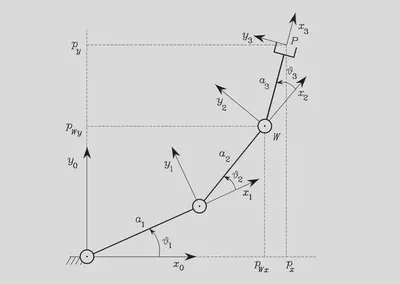
Assuming that we know $(p_{Wx} , p_{Wy})$, $a_1$ and $a_2$. We need to solve $\vartheta_1$ and $\vartheta_2$.

2.1. Geometry Solution

Based on geometry knowledge, we can get $$ p_{Wx}^2 + p_{Wy}^2 = a_1^2 + a_2^2 - 2a_1a_2\cos(180^{\circ} - \vartheta_2) $$

Then, we have $$ \cos \vartheta_2 = \frac{p_{Wx}^2 + p_{Wy}^2 - a_1^2 - a_2^2}{2a_1a_2} $$

According to The Law of Cosines $\cos A=(b²+c²-a²)/2bc$ , we set the angle between $x_1$ and $\vec{p}_W = [p_{Wx} , p_{Wy} , 0]$ is $\psi$, then have $$ \cos \psi = \frac{p_{Wx}^2 + p_{Wy}^2 + a_1^2 - a_2^2}{2a_1\sqrt{p_{Wx}^2 + p_{Wy}^2}} $$

We get $$ \vartheta_1 = \begin{cases} atan2(p_{Wy},p_{Wx}) + \psi & \vartheta_2 < 0^{\circ} \\ atan2(p_{Wy},p_{Wx}) - \psi & \vartheta_2 > 0^{\circ} \end{cases} (0^{\circ} < \psi < 180^{\circ}) $$

2.2. Algebraic Solution

Now, we show the homogeneous transformation matrixs, $$ \begin{aligned} T_2^0 &= T_1^0T_2^1 \\ &= \left[ \begin{matrix} \cos \vartheta_1 & -\sin \vartheta_1 & 0 & a_1\cos \vartheta_1 \\ \sin \vartheta_1 & \cos \vartheta_1 & 0 & a_1\sin \vartheta_1 \\ 0 & 0 & 1 & 0 \\ 0 & 0 & 0 & 1 \end{matrix} \right] \left[ \begin{matrix} \cos \vartheta_2 & -\sin \vartheta_2 & 0 & a_2\cos \vartheta_2 \\ \sin \vartheta_2 & \cos \vartheta_2 & 0 & a_2\sin \vartheta_2 \\ 0 & 0 & 1 & 0 \\ 0 & 0 & 0 & 1 \end{matrix} \right] \\ &= \left[ \begin{matrix} \cos (\vartheta_1 + \vartheta_2) & -\sin (\vartheta_1 + \vartheta_2) & 0 & a_2\cos (\vartheta_1 + \vartheta_2) + a_1 \cos \vartheta_1 \\ \sin (\vartheta_1 + \vartheta_2) & \cos (\vartheta_1 + \vartheta_2) & 0 & a_2\sin (\vartheta_1 + \vartheta_2) + a_1 \sin \vartheta_1 \\ 0 & 0 & 1 & 0 \\ 0 & 0 & 0 & 1 \end{matrix} \right] \\ &= \left[ \begin{matrix} \cos \phi & -\sin \phi & 0 & p_{Wx} \\ \sin \phi & \cos \phi & 0 & p_{Wy} \\ 0 & 0 & 1 & 0 \\ 0 & 0 & 0 & 1 \end{matrix} \right] \end{aligned} $$

We can know $$ \begin{aligned} p_{Wx}^2 + p_{Wy}^2 &= (a_2\cos (\vartheta_1 + \vartheta_2) + a_1 \cos \vartheta_1)^2 + (a_2\sin (\vartheta_1 + \vartheta_2) + a_1 \sin \vartheta_1)^2 \\ &= a_2^2 \cos^2 (\vartheta_1 + \vartheta_2) + a_1^2 \cos^2 \vartheta_1 + 2 a_1 a_2 \cos (\vartheta_1 + \vartheta_2) \cos \vartheta_1 + a_2^2 \sin^2 (\vartheta_1 + \vartheta_2) + a_1^2 \sin^2 \vartheta_1 + 2 a_1 a_2 \sin (\vartheta_1 + \vartheta_2) \sin \vartheta_1 \\ &= a_1^2 + a_2^2 + 2 a_1 a_2 \cos \vartheta_2 \end{aligned} $$

We get $$ \cos \vartheta_2 = \frac{p_{Wx}^2 + p_{Wy}^2 - a_1^2 - a_2^2}{2a_1a_2} $$

If $\cos \vartheta_2 > 1$ or $\cos \vartheta_2 < -1$: too far for the manipulator to reach.
If $-1 \leq \cos \vartheta_2 \leq 1$: two solutions.

Now, we have known $\vartheta_2$, $a_1$ and $a_2$. So we have $$ \begin{aligned} p_{Wx} &= a_2\cos (\vartheta_1 + \vartheta_2) + a_1 \cos \vartheta_1 \\ &= (a_1 + a_2 \cos \vartheta_2)\cos \vartheta_1 + (-a_2 \sin \vartheta_2)\sin \vartheta_1 \\ p_{Wy} &= a_2\sin (\vartheta_1 + \vartheta_2) + a_1 \sin \vartheta_1 \\ &= (a_1 + a_2 \cos \vartheta_2)\sin \vartheta_1 + (a_2 \sin \vartheta_2)\cos \vartheta_1 \end{aligned} $$

Because $\vartheta_2$, $a_1$ and $a_2$ are known, so we set $$ k_1 = a_1 + a_2 \cos \vartheta_2 \\ k_2 = a_2 \sin \vartheta_2 $$

Above functions became (Note: $k_1$ and $k_2$ are constant) $$ p_{Wx} = k_1 \cos \vartheta_1 - k_2 \sin \vartheta_1 \\ p_{Wy} = k_1 \sin \vartheta_1 + k_2 \cos \vartheta_1 $$

Next, we define $$ r = \sqrt{k_1^2 + k_2^2} \\ \gamma = atan2(k_2,k_1) $$

and we have $$ k_1 = r \cos\gamma \\ k_2 = r \sin\gamma $$

then we can get $$ \begin{aligned} \frac{p_{Wx}}{r} &= \frac{k_1 \cos \vartheta_1 - k_2 \sin \vartheta_1}{r} \\ &= \frac{r \cos\gamma \cos\vartheta_1 - r \sin\gamma \sin\vartheta_1}{r} \\ &= \cos\gamma \cos\vartheta_1 - \sin\gamma \sin\vartheta_1 \\ &= \cos(\gamma + \vartheta_1) \end{aligned} $$

in the same way $$ \frac{p_{Wy}}{r} = \sin(\gamma + \vartheta_1) $$

finally, we get $$ \gamma + \vartheta_1 = atan2(\frac{p_{Wy}}{r} , \frac{p_{Wx}}{r}) = atan2(p_{Wy} , p_{Wx}) $$

i.e. $$ \vartheta_1 = atan2(p_{Wy} , p_{Wx}) - atan2(k_2 , k_1) $$

2.3. Solve Trigonometric Equations

For example, we assume that there is an equation, $a \cos\theta + b \sin\theta = c$, we need to solve $\theta$.

First, we set $$ \tan(\frac{\theta}{2}) = \mu ,\ \cos(\theta) = \frac{1 - \mu^2}{1 + \mu^2} ,\ \sin(\theta) = \frac{2\mu}{1 + \mu^2} $$

now we have $$ \begin{align} &a \frac{1 - \mu^2}{1 + \mu^2} + b \frac{2\mu}{1 + \mu^2} = c \\ &(a+c)\mu^2 -2b\mu + (c-a) = 0 \end{align} $$

we get

$$ \mu = \frac{b \pm \sqrt{b^2 + a^2 - c^2}}{a+c} $$

2.4. Generic Inverse Kinematics Algorithm

2.4.1. Introduction

Write a MATLAB function IK.m to solve for the iterative Inverse Kinematics of a given robot. The inputs of this function should be:

DH parameters: $n × 4$ matrix which consists of DH parameters.
joint type: n-dimensional vector which describes joint types (0 for revolute and 1 for prismatic).
q: n-dimensional vector of joint variables specifying the robot’s configuration.
desired position: desired position of the robot’s end-effector. This is $2 \times 1$ vector for a planar robot and $3 \times 1$ vector for a spatial robot.
desired orientation: desired orientation of the robot’s end-effector. This is a scalar for a planar robot and a $3 \times 1$ vector for a spatial robot. Use roll-pitch-yaw angles for 3D robots.

IK can be implemented using the Jacobian Transpose to compute the inverse of the Jacobian matrix. The output of the IK function should be:

a matrix including the robot’s joint variables for each iteration.

Note that, this function solve the IK problem iteratively. So, you need to define appropriate terminating conditions for both maximum iterations and accuracy of the final result. When updating joint variables, consider multiplying by a small gain in order to let the algorithm converge. Use the script IK_test.m to define your robot, solve the IK problem, and visualize how the robot achieves the desired end-effector pose.

2.5. Theoretical Derivation

2.5.1. Geometric Jacobian

As we know, for Geometric Jacobian $$ v_e = \left[ \begin{matrix} \dot{p}_e \\ \dot{w}_e \end{matrix} \right] = J(q)\dot{q} $$

where $J = \left[\begin{matrix} J_P \\ J_O \end{matrix} \right]$.

So we have

$$ \dot{q} = J^{-1}v_e $$

that is $$ [\Delta \vartheta_1, \Delta \vartheta_2 ... \Delta \vartheta_n] = J^{-1} [\Delta p_x, \Delta p_y, \Delta p_z, \Delta w_x, \Delta w_y, \Delta w_z] $$

i.e. $$ [\frac{\vartheta_1}{t}, \frac{\vartheta_2}{t} ... \frac{\vartheta_n}{t}] = J^{-1} [\frac{p_x}{t}, \frac{p_y}{t}, \frac{p_z}{t}, \frac{w_x}{t}, \frac{w_y}{t}, \frac{w_z}{t}] $$

where $\vartheta$ corresponds to the angle of joints, $p$ and $w$ corresponds to the position and orientation of the end-effector.

2.5.2. Analytical Jacobian

For Analytical Jacobian $$ \dot{x}_e = \left[ \begin{matrix} \dot{p}_e \\ \dot{\phi}_e \end{matrix} \right] = \left[\begin{matrix} J_P(q) \\ J_\phi(q) \end{matrix} \right] \dot{q} = J_A(q)\dot{q} $$

So we have

$$ \dot{q} = J_A^{-1}\dot{x}_e $$

that is $$ [\Delta \vartheta_1, \Delta \vartheta_2 ... \Delta \vartheta_n] = J^{-1} [\Delta p_x, \Delta p_y, \Delta p_z, \Delta \psi, \Delta \vartheta, \Delta \varphi] $$

i.e. $$ [\frac{\vartheta_1}{t}, \frac{\vartheta_2}{t} ... \frac{\vartheta_n}{t}] = J^{-1} [\frac{p_x}{t}, \frac{p_y}{t}, \frac{p_z}{t}, \frac{\psi}{t}, \frac{\vartheta}{t}, \frac{\varphi}{t}] $$

where $\vartheta$ corresponds to the angle of joints, $p$ corresponds to the position of the end-effector, $[\psi , \vartheta , \varphi]$ corresponds to the [yaw, pitch, yaw](RPY Angles system) respectively.

2.5.3. Jacobian Pseudo-inverse (generalized inverse)

Set the size of Jacobian is $[n,m]$, them we have:

when $n>m$, we use left generalized inverse $$ A^\dagger_{left} = (A^\mathsf{T}A)^{-1}A^\mathsf{T} $$
when $n

2.5.4. Kinematic Singularities

For Kinematic Singularities, we set a small value of $k$ to let the algorithm converge. (Damped least squares) $$ J^* = J^\mathsf{T}(J J^\mathsf{T} + k^2I)^{-1} $$

normally, we set $k = 0.01$.

2.6. Algorithm Overview

se set: $\theta_k:$ initial joint angles $p_{des}:$ desired position $o_{des}:$ desired orientation $t:$ Hypothetical robot movement time

We get the homogeneous transformation matrix $T_k$ form $\theta_k$.
Calculate the position $p_k$ and oritention $w_k$ of the end-effector.
We approximate the velocity of end effector movement $v_k = ([p_{des}, o_{des}] - [p_k, w_k]) ./ t$
Get Joint Angle Increment $\Delta \theta = J_k^{-1} * v_k$
Update joint angles $\theta_{k+1} = \theta_k + \Delta \theta$
Calculation error, determining whether to continue iterating.

2.7. Demo Codes

IK.m

Below codes show the inverse kinematics algorithm.

function Q = IK(DH_params, jtype, q, pdes, odes)
% IK calculates the inverse kinematics of a manipulator
% Q = IK(DH_params, jtype, q, pdes, odes) calculates the joint
% values of a manipulator robot given the desired end-effector's position
% and orientation by solving the inverse kinematics, iteratively.  The
% inputs are DH_params, jtype and q, pdes, and odes.  DH_params is
% nx4 matrix including Denavit-Hartenberg parameters of the robot.  jtype
% and q are n-dimensional vectors.  jtype describes the joint types of the
% robot and its values are either 0 for revolute or 1 for prismatic joints.
% q is the joint values.  pdes and odes are desired position and
% orientation of the end-effector.  pdes is 2x1 for a planar robot and 3x1
% for a spatial one.  odes is a scalar for a planar robot and a 3x1 vector
% for a 3D robot.  Orientation is defined as roll-pitch-yaw angles.  Use
% Jacobian Transpose to compute the inverse of the Jacobian.

n = size(q,1);  % robot's DoF
% consistency check
if (n~=size(DH_params,1)) || (n~=size(jtype,1))
    error('inconsistent in dimensions');
end

% robot's dimension (planar or spatial)
dim = size(pdes,1);
if ~((dim==2) || (dim==3))
    error('size of pdes must be either 2x1 for a planar robot or 3x1 for a spatial robot');
end

% check the size of orientation parameter
if dim==2
    if size(odes,1)~=1
        error('desired orientation must be scalar for a planar robot');
    end
else
    if size(odes,1)~=3
        error('desired orientation must be 3x1 for a spatial robot');
    end
end

%% iterative inverse kinematics


Q = q;  % joint angle
thetaK = q;  % initial joint angle
time = 100;
iTime = 0;
single = 1; % if value is 1, continue to iterate

% Calculate the oritention of the end effector in the current stage
[TCur_k,J_k] = FK(DH_params, jtype, q);
o_e = oEnd(TCur_k(1:3,1:3));

% Approximate end-effector velocity, determine the direction of movement
dX = ([pdes; odes] - [TCur_k(1:3,4); o_e]) ./ time;


JTranspose = IKJ(J_k);
dO = JTranspose *  dX; % Variation of joint angles

while single

    iTime = iTime +1;
    thetaK1 = dO + thetaK;

    % Calculate the oritention of the end effector in the next stage
    [TCur_k1,J_k1] = FK(DH_params, jtype, thetaK1);
    o_e1 = oEnd(TCur_k1(1:3,1:3));

    % calculate the error
    e = sum(sum(abs([TCur_k1(1:3,4); o_e1] - [pdes; odes])));
    if e<0.1 || iTime>= time
        single = 0; % stoping iterating
    end

    thetaK = thetaK1;
    JTranspose = IKJ(J_k1);
    dO = JTranspose *  dX; % Variation of joint angles

    Q = [Q,thetaK];
end

end



%% IKJ
% Pseudo-Inverse Matrix Solving
function JTranspose = IKJ(J)

[n,m] = size(J);
k = 0.01; % Avoid singular solutions

if n>m
    JTranspose = (J' * J + k^2 .* eye(m,m)) \ J';
else
    JTranspose = J' / (J  * J' + k^2 .* eye(n,n));
end

end


%% oEnd
% Convert rotation matrix to angles of end effector
function o = oEnd(R)

o = zeros(3,1);

% x
o(3) = atan2(R(2,1), R(1,1));
% y
o(2) = atan2(-R(3,1), sqrt(R(3,2)^2 + R(3,3)^2));
% z
o(1) = atan2(R(3,2), R(3,3));
end

IK_test.m